Category: Technical

Introduction

The accepted way to determine Depth of field has not changed  for many years but with the progress of cultural heritage photography, and how that photography is viewed, it may well mean you need to give more thought to how you calculate it in the future.

How Depth of Field is calculated

Depth of field is calculated from the following formula:

d = 2NCD²/ f²

Equation 1.

Where:

N = f/number

C = circle of confusion

D = focus distance

f = focal length of the lens

The determining factor here is the circle of confusion (C), as the other 3 parameters will remain the same for any given shot.

Circle of confusion is taken as the maximum diameter a spot can be “blurry” but still appear sharp to the viewer and this is commonly determined with the viewer at a distance of 25cm viewing a print approximately 25 cm x 20 cm.

As an average person can determine around 100 points per cm at this distance (or 5 line pairs per mm), this approximates to a circle of confusion with a diameter of 0.2mm.

However this is the diameter of a blurry point that will appear sharp to us on print and it is from this that the circle of confusion that will be acceptable falling on the camera’s sensor is calculated.

For an example let’s look at a Canon 7D MarkII which has the following specifications:

Sensor Dimensions: 22.4 x 15mm

Pixel dimensions: 5472 x 3648 px

The enlargement required to produce a 25 x 20 cm print is given by the length of the print divided by the length of the sensor:

250mm / 22.4mm = 11.16 enlargement.

With the enlargement required we can calculate the circle of confusion by taking the required print circle of confusion, 0.2mm, and dividing it by the enlargement required. In the case of a Canon 7D Mark II, 11.16:

0.2mm / 11.16 = 0.018mm or 18µm

Now we have the circle of confusion required for our sensor to produce a sharp image viewed on our print the depth of field can be calculated.

To make things easy in our example we are going to use a 100mm lens, with an aperture of f/11 at a focal distance of 1m. If we put these figures into equation 1, we get:

d = 2 x 11 x 0.018 x (1000²) / 100²   =   39.6mm

Therefore the depth of field is 39.6mm from front to back in the scene that will appear sharp on the 25 x 20 cm print.

The Problem

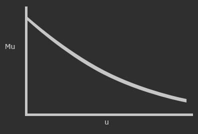
The problem is that with the increased popularity of viewing “zoomed” images on screen the circle of confusion that would be acceptable with a depth of field of 39.6mm in our example will appear blurry when viewed at 100％ on screen.

To demonstrate the problem take a look at the illustration below. This shows just how great an area a circle of confusion of 0.018µm diameter will be recorded on the sensor of the Canon 7D MarkII which has a pixel width of about 4.1µm.

It is this circle of confusion that is usually used in the calculation of depth of field. What needs to be calculated is a circle of confusion that will provide a sharp image when viewed on screen at 100％.

Ideally a circle of confusion equal to the width of the pixel would provide the basis for the depth of field calculation.

In this case the depth of field for the same shot as the example earlier becomes:

d = 2 x 11 x 0.0041 x (1000²) / 100²   = 9.02mm

Now the depth of the scene that will be in focus when viewed has reduced significantly from 39.6mm to 9.02mm, a difference of 30.58mm, or a 77％ reduction.

For practical purposes a useful rule of thumb is to use a circle of confusion equivalant to double the pixel width on the sensor. In the case of the Canon 7D MarkII this would be 0.0082µm.

This would result in the following depth of field in our example:

d = 2 x 11 x 0.0082 x (1000²) / 100²   = 18.04mm

This results in a significantly greater depth of field than using the pixel width, 9.02mm, but still significantly less than using the more traditional calculation for the circle of confusion, 39.60mm.

Summary

• The next time you look at the depth of field scale on your lens give some thought to how your image will be viewed. They may not be relevant.
• As the pixel width decreases on the sensors to accommodate more pixels the acceptable sharpness and depth of field will be affected to a greater extent if the images are to be viewed at 100％ on a display.